Online Scaling and Preprocessing

Feature Scaling: Mean-STD vs. Mean-MAD

This module provides two normalization strategies with different assumptions about the data distribution and sensitivity to outliers.

Mean-STD Scaling

Transforms each feature as: z = (x - mean) / std and hence

Centers data around 0 using the arithmetic mean.
Scales to unit variance using standard deviation.
Works best when features are approximately Gaussian and outliers are limited.
Sensitive to extreme values, since both mean and std are strongly affected by them.

Mean-MAD

Transforms each feature as: zt = (x - mean) / MAD where:

MAD = mean(|x - mean|) is the mean absolute deviation from the mean.
Reduces the influence of outliers compared to standard deviation-based scaling.
Better for heavy-tailed, skewed, or contaminated datasets.
May be less efficient than mean-STD scaling on normal data
Does not track exactly online, but only approximately (see below)

Choosing between them

Use OnlineScalerfor well-behaved, near-normal features and models that assume standardized Gaussian-like inputs.
Use OnlineMeanAbsoluteDeviationScaler when outliers are common or feature distributions are non-Gaussian and you want more stable scaling factors.

Online Tracking Behaviour

The mean can be tracked online exactly through a simple recursion formula.

Based on this and Welford's formula (see e.g. here), the variance and weighted variances can be tracked exactly. The variance is defined as: $$\text{Var}_n = \frac{1}{n} \sum_{i=1}^{n} (x_i - \mu_n)^2$$ and the following key identity allows online update: $$\sum_{i=1}^{n} (x_i - \mu_n)^2 = \sum_{i=1}^{n-1} (x_i - \mu_{n-1})^2 + n(\mu_n - \mu_{n-1})^2$$ However, for the mean absolute deviation from the mean, no such closed-form $\mathcal{O}(1)$ update exists.

The reason for this is explained in the following quick example. The true MAD after $n$ updates is defined as: $$\text{MAD}_n = \frac{1}{n} \sum_{i=1}^{n} |x_i - \mu_n| \quad \text{where} \quad \mu_n = \frac{1}{n} \sum_{i=1}^{n} x_i$$ But online tracking gives you: $$\text{MAD}_{\text{online}} = \frac{1}{n} \sum_{i=1}^{n} |x_i - \mu_i| \quad \text{where} \quad \mu_i = \text{mean after } i \text{ points}$$ Where each $x_i$ is measured against a different mean ($\mu_i$ instead of $\mu_n$). and there is no: $$\sum_{i=1}^{n} |x_i - \mu_n| \neq \sum_{i=1}^{n-1} |x_i - \mu_{n-1}| + [\text{simple update term}]$$ The absolute value prevents algebraic simplification. We cannot incrementally update MAD when the mean changes without revisiting all previous points.

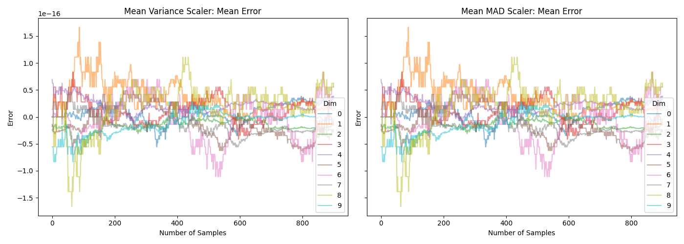
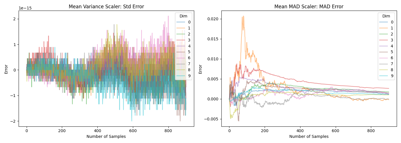
The difference can also be seen in the following two plots. Note that the $y$-axis in the lower plot is very different.

Difference in mean

Difference between dispersion (standard deviation and mean absolute deviation)

Which can be generated with the following script:

import numpy as np
import scipy.stats as stats
import matplotlib.pyplot as plt
from ondil.scaler import (
    OnlineMeanAbsoluteDeviationScaler,
    OnlineScaler,
)

INIT_SIZE = 100
SIZE = 1000
DIMS = 10
SEED = 42

rng = np.random.default_rng(SEED)

mean_var = OnlineScaler()
mean_mad = OnlineMeanAbsoluteDeviationScaler()

X = rng.standard_normal(size=(SIZE, DIMS))
w = rng.uniform(0.1, 1.0, SIZE)

true_mean = np.zeros((SIZE - INIT_SIZE + 1, DIMS))
pred_mean = np.zeros((SIZE - INIT_SIZE + 1, 2, DIMS))

true_dispersion = np.zeros((SIZE - INIT_SIZE + 1, 2, DIMS))
pred_dispersion = np.zeros((SIZE - INIT_SIZE + 1, 2, DIMS))

for i, t in enumerate(range(INIT_SIZE, SIZE + 1)):
    if i == 0:
        mean_var.fit(X[:t], sample_weight=w[:t])
        mean_mad.fit(X[:t], sample_weight=w[:t])
    else:
        mean_var.update(X[t - 1 : t], sample_weight=w[t - 1 : t])
        mean_mad.update(X[t - 1 : t], sample_weight=w[t - 1 : t])

    true_mean[t - INIT_SIZE, :] = np.average(X[:t], axis=0, weights=w[:t])
    pred_mean[t - INIT_SIZE, 0, :] = mean_var.mean_
    pred_mean[t - INIT_SIZE, 1, :] = mean_mad.mean_

    true_dispersion[t - INIT_SIZE, 0, :] = (
        np.average((X[:t] - true_mean[t - INIT_SIZE, :]) ** 2, axis=0, weights=w[:t])
        ** 0.5
    )
    true_dispersion[t - INIT_SIZE, 1, :] = np.average(
        np.abs(X[:t] - true_mean[t - INIT_SIZE, :]), axis=0, weights=w[:t]
    )
    pred_dispersion[t - INIT_SIZE, 0, :] = mean_var.dispersion_
    pred_dispersion[t - INIT_SIZE, 1, :] = mean_mad.dispersion_

# %%
titles = ["Mean Variance Scaler: Mean Error", "Mean MAD Scaler: Mean Error"]
fig, axes = plt.subplots(1, 2, figsize=(14, 5), sharex=True, sharey=True)
for i in range(2):
    axes[i].plot(
        true_mean - pred_mean[:, i, :],
        alpha=0.5,
        label=range(DIMS),
    )
    axes[i].set_title(titles[i])
    axes[i].set_xlabel("Number of Samples")
    axes[i].set_ylabel("Error")
    axes[i].legend(title="Dim")
plt.tight_layout()
plt.show(block=False)

# %%
fig, axes = plt.subplots(1, 2, figsize=(14, 5), sharex=True, sharey=False)
titles = ["Mean Variance Scaler: Std Error", "Mean MAD Scaler: MAD Error"]

for i in range(2):
    axes[i].plot(
        true_dispersion[:, i, :] - pred_dispersion[:, i, :],
        alpha=0.5,
        label=range(DIMS),
    )
    axes[i].set_title(titles[i])
    axes[i].set_xlabel("Number of Samples")
    axes[i].set_ylabel("Error")
    axes[i].legend(title="Dim")
plt.tight_layout()
plt.show(block=False)

API Reference

ondil.scaler.OnlineScaler

Bases: OndilEstimatorMixin, TransformerMixin, BaseEstimator

dispersion_ `property`

dispersion_

Scale factor for the scaled variables.

init

__init__(
    forget: float = 0.0, to_scale: bool | ndarray = True
)

The online scaler allows for incremental updating and scaling of matrices.

Parameters:

forget (float, default: 0.0 ) –

The forget factor. Older observations will be exponentially discounted. Defaults to 0.0.
to_scale (bool | ndarray, default: True ) –

The variables to scale. True implies all variables will be scaled. False implies no variables will be scaled. An np.ndarray of type bool or int implies that the columns X[:, to_scale] will be scaled, all other columns will not be scaled. Defaults to True.

fit

fit(
    X: ndarray,
    y: None = None,
    sample_weight: ndarray | None = None,
) -> OnlineScaler

Fit the OnlineScaler() Object for the first time.

Parameters:

X (ndarray) –

Matrix of covariates X.
y (None, default: None ) –

Not used, present for compatibility with sklearn API. Defaults to None.
sample_weight (ndarray, default: None ) –

Weights for each sample. Defaults to None (uniform weights).

update

update(X: ndarray, y=None, sample_weight: ndarray = None)

Update the OnlineScaler() for new rows of X.

Parameters:

X (ndarray) –

New data for X.
y (None, default: None ) –

Not used, present for compatibility with sklearn API. Defaults to None.
sample_weight (ndarray, default: None ) –

Weights for each sample. Defaults to None (uniform weights).

transform

transform(X: ndarray) -> np.ndarray

Transform X to a mean-std scaled matrix.

Parameters:

X (ndarray) –

X matrix for covariates.

Returns:

ndarray –

np.ndarray: Scaled X matrix.

inverse_transform

inverse_transform(X: ndarray) -> np.ndarray

Back-transform a scaled X matrix to the original domain.

Parameters:

X (ndarray) –

Scaled X matrix.

Returns:

ndarray –

np.ndarray: Scaled back to the original scale.

ondil.scaler.OnlineMeanAbsoluteDeviationScaler

Bases: OnlineScaler

Robust online scaler using mean absolute deviation (MAD)

This scaler is more robust to outliers than the standard OnlineScaler which uses mean and standard deviation for scaling. The OnlineMeanAbsoluteDeviationScaler uses the mean and mean absolute deviation (MAD) for scaling, which can provide better performance in the presence of outliers.

Note

The MAD does not have a closed-form solution and is estimated using an online update rule. As a result, the tracking of the MAD is approximate. The mean is tracked exactly, but the MAD estimation can deviate, especially in the early stages of fitting or with small sample sizes. For more details on the estimation of the MAD and its properties see the documentation and the tests for this scaler.

dispersion_ `property`

dispersion_

Dispersion of the scaled variables (equal to MAD for this scaler).

fit

fit(
    X: ndarray,
    y: None = None,
    sample_weight: ndarray | None = None,
) -> OnlineMeanAbsoluteDeviationScaler

Fit the OnlineMeanAbsoluteDeviationScaler() object for the first time.

update

update(X: ndarray, y=None, sample_weight: ndarray = None)

Update the OnlineMeanAbsoluteDeviationScaler() for new rows of X.

transform

transform(X: ndarray) -> np.ndarray

Transform X to a mean-MAD scaled matrix.

inverse_transform

inverse_transform(X: ndarray) -> np.ndarray

Back-transform a mean-MAD scaled X matrix to the original domain.

update_transform

update_transform(
    X: ndarray, y=None, sample_weight: ndarray = None
) -> np.ndarray

Convenience method to update the scaler and transform the new data in one step.

Online Scaling and Preprocessing

Feature Scaling: Mean-STD vs. Mean-MAD

Mean-STD Scaling

Mean-MAD

Choosing between them

Online Tracking Behaviour

API Reference

ondil.scaler.OnlineScaler

dispersion_ property

__init__

fit

update

transform

inverse_transform

ondil.scaler.OnlineMeanAbsoluteDeviationScaler

dispersion_ property

fit

update

transform

inverse_transform

update_transform

dispersion_ `property`

init

dispersion_ `property`